CS 240: Lecture 7 – Amortized Analyis of ArrayList
Dear students:
Today we begin our application of complexity analysis to real live data structures that software developers use everyday. The first data structure to go under the microscope is the array-based list. Before that, though, we need to discuss one alternative view of the complexity classes.
Limit Definitions
Last week we looked at ways of proving that growth functions were $O$, $\Omega$, or $\Theta$ of some representive growth function by finding constants that bound the growth function above and below. Sometimes finding constants is tedious work. On such occasions, you might prefer to calculate this ratio:
If the limit converges, then the value $c$ tells us what set the growth function belongs to:
We’re not going to prove this. Sorry.
Let’s apply this strategy in a few examples. Consider $T(n) = n^3 + 2n$ and $f(n) = n^3$. We solve the limit:
Since $c = 1$, we have $\Theta$ membership.
Consider $T(n) = \frac{n}{2}$ and $f(n) = n^2$. We solve the limit:
Since $c = 0$, we have $O$ membership, but not the others.
Consider $T(n) = 2^n$ and $f(n) = 3^n$. We solve the limit:
Since $c = 0$, we have $O$ membership, but not the others.
We’ll work through $T(n) = 6n + \sqrt{n}$ and $f(n) = 2n$ as a peer instruction exercise.
ArrayList
We now move on to a discussion of data structures. For the rest of the semester we will be dragging various data structures onto the stage and discussing their complexity. Our first subject is an array-based list.
Your book introduces its own flavor of an array-based list called AList. What is the output of this program?
List<Integer> numbers = new AList<>();

for (int i = 0; i < 10000; i++) {
  numbers.append(i);
}

System.out.println(numbers.length());
It prints 10. That’s because the book has a made a design decision that makes it very different from Java’s ArrayList. The AList is a list of fixed size. The fixed size defaults to 10.
What’s the complexity of AList.append?
// Append "it" to list
public boolean append(E it) {
  if (listSize >= maxSize) {
    return false;
  }
  listArray[listSize++] = it;
  return true;
}
There’s no loop here nor any calls to expensive operations. This is a constant-time algorithm.
What is the output of this program?
List<Integer> numbers = new ArrayList<>();

for (int i = 0; i < 10000; i++) {
  numbers.add(i);
}

System.out.println(numbers.size());
This code prints 10000, as you’d expect. Java’s ArrayList does not have a fixed size. How does it manage this? It starts off with a small array of a certain length. OpenJDK starts off with 10. There aren’t any items in this array initially, so the list itself has size 0, even though the array has length 10. To track the size of the list, the ArrayList holds an extra int.
As the client calls add, the array fills up. Eventually the size of the list matches its capacity. If the client calls add on a full list, a new and bigger array is created, and all of the elements from the previous array are copied over to it. Here’s how I might implement the add method:
public void add(T item) {
  if (size >= items.length) {
    grow();
  }
  items[size] = item;
  ++size;
}

private void grow() {
  E[] biggerItems = (E[]) new Object[items.length * 2];
  for (int i = 0; i < size; ++i) {
    biggerItems[i] = items[i];
  }
  items = biggerItems;
}
This add method is different from AList.add. What can we say about it’s complexity? The cost depends on how many items have already been added to the list, so we have to look at more than just the parameter item. When the list is full, we will have to copy over all elements of the list to a new array. The worst case is therefore $\Theta(n)$. However, if the list is not full, the algorithm is constant time. The best case is therefore $\Theta(1)$.
This split leads to an interesting problem. How do we analyze this algorithm?
public static void addNumbers(int n) {
  ArrayList<Integer> nums = new ArrayList<>();

  for (int i = 0; i < n; i++) {
    nums.add(i); // Best case Theta(1), worst case Theta(n)
  }
}
The client doesn’t exactly know that this expansion is happening. However, when I time and plot these calls to add, I see a distinct pattern:
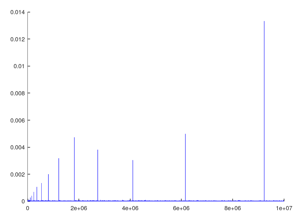
So, is the algorithm above $\Theta(n^2)$? $\Theta(n)$? Or something else?
Amortization
Suppose you ask me what I pay in property taxes each month. What do I answer? This month I didn’t pay anything. Nor will I in October. Come November, however, I’ll be shelling out $1200. In the best case, I pay $0. In the worst case, I pay $1200. In most of our analysis work so far, we’ve favored being pessimistic. However, if I say that I pay $1200 a month in property taxes, that’s overly pessimistic. It’s a misleading exaggeration.
If we know that the worst case is not so frequent, then we should perform a more nuanced analysis. A reasonable solution is to add up what I pay each month of the year and divide by 12 to get an average. This kind of reasoning is called amortized analysis. To amortize is to spread out a cost.
We should use amortized analysis to measure ArrayList.add. Calling it $\Theta(n^2)$ is a borderline lie. To ease the analysis, let’s assume that the array starts off with a single element and doubles in size once it fills. To structure our thinking, we’ll complete this table:
| n | assignment cost | resize cost | total cost | amortized cost |
|---|---|---|---|---|
| 1 | 1 | 0 | 1 | 1 |
| 2 | 1 | 1 | 3 | 1.5 |
| 3 | 1 | 2 | 6 | 2 |
| 4 | 1 | 0 | 7 | 1.75 |
| 5 | 1 | 4 | 12 | 2.4 |
| 6 | 1 | 0 | 13 | 2.167 |
| 7 | 1 | 0 | 14 | 2 |
| 8 | 1 | 0 | 15 | 1.875 |
| 9 | 1 | 8 | 24 | 2.667 |
| … | … | … | … | … |
The cost of adding element $n$ is the cost of adding all the preceding elements, plus the assignment, plus any resizing that needs to be done. Dividing the total cost by the number of times add has been called gives us the amortized cost of each add.
In general, element $n$ will have these costs:
When we average this out, we see that each add has a constant cost of around 3 operations. Thus we say that adding to an ArrayList is $\Theta(1)$, that it has amortized constant time. That’s pretty good. In fact, it’s just as good as AList, which used a fixed-size array. Even the ArrayList documentation proudly declares this.
TODO
- Submit a muddiest point today.
- Keep working on PA1. Run into issues now, while there’s time to address them.
See you next time.

P.S. It’s time for a haiku!
That meal filled me up
Time to find a new body
I know, it sounds growth