CS 240: Lecture 38 – Graph Algorithms
Dear students:
I don’t know about you, but my mind has been elsewhere. Our routine striving was cut into by a break. I’m glad it did. Sometimes I think that I’ll only have peace when I get all the things done. What a lie that is. I will never be done. And even if something I’m working on gets finished, I won’t have peace afterward, not for long anyway. It’s better that breaks just interrupt us without waiting for a convenient time.
We pick up our conversation of algorithms and data structures with a couple of tricks for finding meaningful paths through graphs. First we’ll find a path that navigates through a prerequisite chain. Second we’ll find the shortest path from a vertex to another. These problems are pretty easy for humans to solve visually when the number of vertices is small. Don’t be deceived. As with every other topic in this class, we must assume that the size of our data structure will exceed our capacity to deal with it. Yet when we introduce the topic, we use small examples.
Topological Sort
Imagine a series of tasks in a multi-task process. Some tasks must be completed before others. For example, maybe you’re planning a space flight. You’ve got to get some new o-rings before you assemble the solid rocket booster before you install the booster. Other tasks can be scheduled more freely, like celebrating a successful launch with a glass of Blue Powerade. They can happen any time after earlier stages. You can find a path through this process by making each stage a vertex. If a stage is a prerequisite for another, then there’s a directed and unweighted edge from the prerequisite to its successor. Then you run a topological sort on the graph.
The Greek word topos means place. The topological sort orders the vertices by their place in the prerequisite chain, not by any numeric value. The algorithm can be implemented a couple of different ways. We can run a depth-first traversal, chasing out the longest prerequisite chain in the graph and adding its vertices in backward order and branching recursively through the neighbors. A pseudocode implementation might look like this:
function topologicalSort(graph g)
  for each vertex v
    mark v as unvisited
  order = []
  for each vertex v
    if v is unvisited
      depthTraverse(g, v, order)

function depthTraverse(graph g, vertex v, list order)
  mark v as visited
  for each neighbor n
    if n is unvisited
      depthTraverse(g, n)
  prepend v to order
Alternatively, if we wish to avoid the recursion, we can implement this with a breadth-first traversal. This implementation works by keeping a count of how many incoming edges each vertex has from unvisited vertices. When that number goes to 0, a vertex’s prerequisites have been visited and thus it is safe to visit the vertex. Here’s how it might be implemented in pseudocode:
function topologicalSort(graph g)
  create queue
  order = []

  for each vertex v
    inCounts[v] = 0

  for each vertex v
    for each neighbor n
      increment inCounts[n]

  for each vertex v
    if inCounts[v] is 0
      enqueue v

  while queue isn't empty
    v = dequeue
    append v to order
    for each neighbor n
      decrement inCounts[n]
      if inCounts[n] is 0
        enqueue n
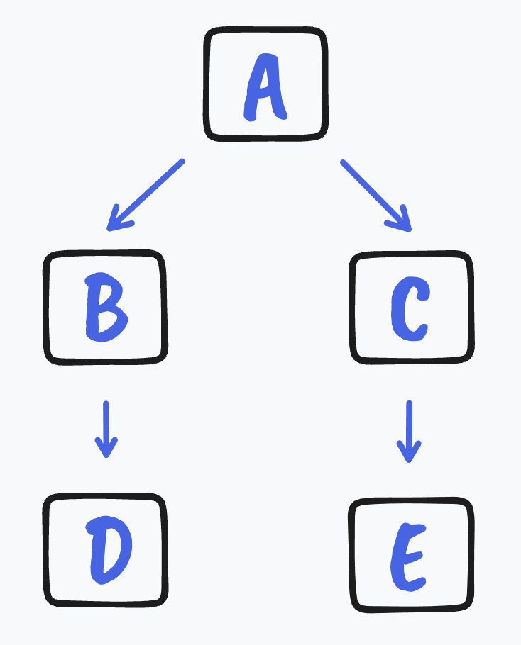
There are more legal topological sorts than these deterministic algorithms will generate. Consider this graph:

How many possible topological sorts are there for this graph? We’ll answer this as a peer instruction exercise.
Shortest Paths
The second algorithm we’ll look at today finds the quickest route from a starting vertex to all the other vertices in the graph. This algorithm was invented by Edsger Dijkstra, an opinionated computer scientist from the Netherlands. It works by maintaining a record of how distant each vertex is. Initially all vertices are infinitely far away, except for the starting vertex, which has a distance of 0. It advances to the next nearest vertex. If that vertex makes reaching other vertices cheaper, then those vertices’ distances are lowered. Then it advances again and again, until all vertices have been visited.
To actually trace out a path, the algorithm must keep track of which vertex provided the cheapest route. We walk this list of predecessors backward to generate the complete path.
function shortestPaths(graph g, vertex from, int[] distances, vertex[] predecessors)
  for each vertex v
    distances[v] = infinity
    predecessors[v] = null
    mark v as unvisited

  distances[from] = 0
  repeat g.vertices.size
    v = find closest unvisited vertex
    mark v as visited
    if distances[v] is infinity
      return as there's no way to reach any more vertices

    for each neighbor n
      distanceViaV = distances[v] + g.weight(v, n)
      if distances[n] > distanceViaV
        distances[n] = distanceViaV
        predecessors[n] = v
To find the shortest path to a particular destination, we trace backward through the predecessors list, starting at the at destination and stopping at from.
Exercises
For the remainder of our time, we will work through an exercise on Dijkstra’s algorithm.
TODO
You have some work to do before the next class:
- Keep working on PA4. It is due on Wednesday.
- Complete the quizzes by the end of today.
- Submit the lab by the end of today.
- There are no more OpenDSA readings.
See you next time.

P.S. It’s time for a haiku!
Course N won’t make sense
Not until course N + 1
Thus post-requisites